SQL is a powerful and essential tool in the development and maintenance of relational database management systems. In fact, it is used to store and manipulate data, as well as to query multiple databases simultaneously.
In the previous post, we looked into the key concepts of Database Management Systems (DBMS). In this blog post, we will explore the SQL query language in-depth, focusing primarily on the SQL2 (SQL 92) and SQL3 (SQL 99) standards. We will cover key features and capabilities of the language, including the JOIN family of operators, nested subqueries, set operators, table variables and more.
We will also provide hands-on examples and exercises to help readers practice and apply the concepts being covered. By the end of this post, readers will have a solid understanding of the basics of SQL and be able to use the language to manage and analyze data in a relational database.
Table of Contents
Intro – What is The SQL Language
SQL is a declarative language that is used to manage and manipulate data in relational database management systems. It consists of two main parts: the Data Definition Language (DDL) and the Data Manipulation Language (DML). While DDL includes commands for creating, altering, and deleting tables and other database objects, DML contains statements for querying, inserting, updating, and deleting data.
Unlike other programming languages, SQL is non-procedural, meaning that users specify what data they want from the database, rather than describing how to retrieve it. To achieve this, SQL relies on the query optimizer, a component of the database system that determines the most efficient way to execute a given query.
For instance, the following are some examples of DDL queries, taken from Microsoft’s official documentation:
- The CREATE DATABASE and DROP DATABASE statements are used to create and delete databases, respectively.
- The USE DATABASE statement allows you to switch to a different database within the same server.
- The CREATE TABLE and DROP TABLE statements are used to create and delete tables, respectively. The table definition can include various options and constraints, such as indexes, partitions, and distribution methods.
On the other hand, the following are some examples of DML queries, also taken from Microsoft’s official documentation:
- The SELECT statement is used to retrieve data from one or more tables.
- The INNER JOIN clause is used to combine rows from two or more tables based on a matching column or condition.
- The AS keyword is used to rename a column or expression in the result set.
- The COUNT function is used to count the number of rows in a table or a group of rows based on a given condition.
The SQL Data Manipulation Language
The SQL Data Manipulation Language (DML) consists of a subset of SQL-data statements that modify stored data, such as SELECT, INSERT, UPDATE, and DELETE. These verbs are used to manipulate persistent database objects, such as tables or stored procedures, and are distinct from the Data Definition Language (DDL) in terms of syntax, data types, and expressions.
Although SELECT is traditionally considered part of the DQL (Data Query Language), it is often considered part of the DML in common practice. Additionally, SELECT … INTO … combines selection and manipulation, making it a part of the DML as well.
In general, the Data Manipulation Language is a powerful and useful tool for a variety of purposes. DML can be used to create reports and analyze data, create tables and views, add, delete, or modify data, and control database security. The DML can also be used to create triggers and stored procedures. Overall, the DML is an essential component of the SQL language and is widely used in database management and data analysis.
The SQL Data Definition Language
The Data Definition Language (DDL) is a component of SQL that is used to create, alter, and delete data structures such as tables, views, indexes, and schemas. It is also used to define or redefine constraints on these structures. DDL statements generally include the following: CREATE, ALTER, DROP, RENAME, and TRUNCATE.
Using DDL, a developer or database administrator can define the data type and size of each field in a database table, the structure of the table, and any constraints that the data must follow.
For example, a developer can specify that a field in a table must contain only numbers, or that it must contain a certain range of numbers. This is a powerful tool that helps ensure data integrity and accuracy.
In addition to creating new structures, DDL is also used to modify existing structures. For example, we can use it to add or remove fields, change data types, and rename fields. DDL can also be used to delete existing structures, such as when a project is no longer needed or when a database table needs to be updated. Overall, DDL is an essential component of SQL that is used to define and maintain the structure and organization of data in a database.
The Relational Model
The Relational Model is a widely used concept in database management systems that has a long history dating back more than 35 years. It forms the basis for many commercial database systems and has contributed to the growth of a multi-billion dollar industry.
One of the main benefits of the Relational Model is its simplicity, which makes it easy to query using High-Level Languages. These languages allow us to express queries in a way that is easy to understand, and there are also efficient implementations of both the model and the query languages.
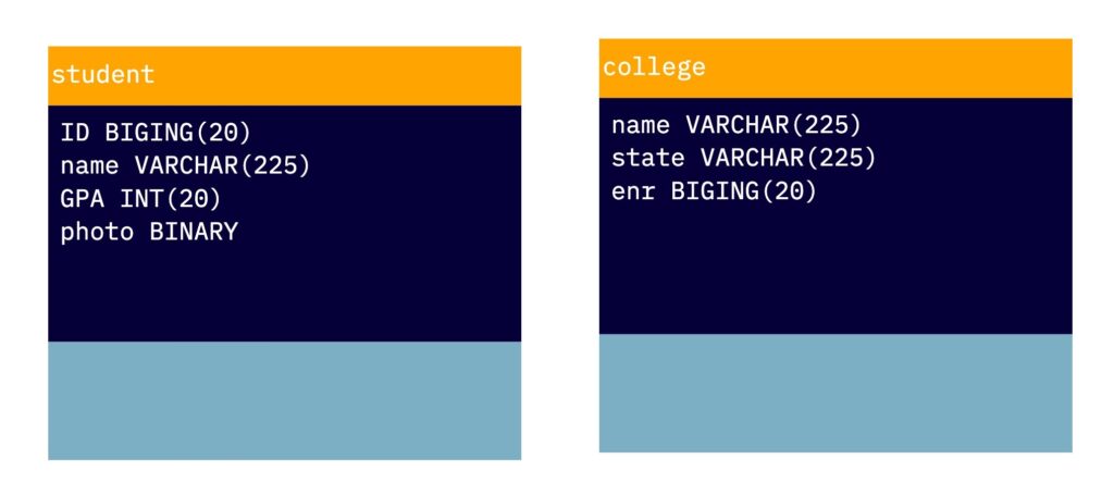
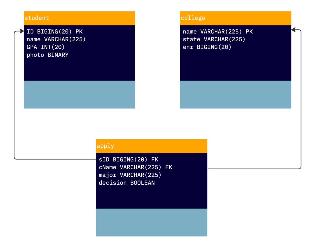
In the Relational Model, data is organized into tables, or relations, which have a set of defined columns, or attributes. For example, in a fictitious database about students applying to colleges, there could be three tables: one for students, one for colleges, and one for applications. Each of these tables holds the related information, and some of the values, such as IDs and names, are used for referring between different relations. We will see more examples of this in the following sections of the post.
The Students Database
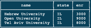
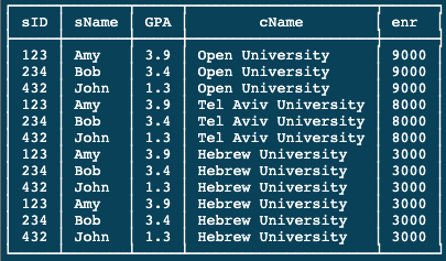
Next, let’s create a database. There is some debate about whether tables should be named using the singular or plural form, but for now, we will use the singular. Each table has a predefined set of attributes, such as sID, name, GPA, and photo for the student table, and name, state, and enrollment (abbreviated as ENR) for the college table.
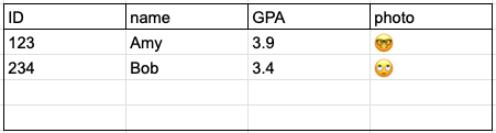
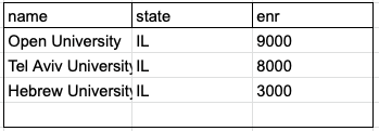
In the diagram below, you can see that the student table has tuples for Amy (sID 123, GPA 3.9, 🤓) and Bob (sID 234, GPA 3.4, 🙄), while the college table has tuples for OUI (state Israel, enrollment 9,000), HUJ (state Israel, enrollment 3,000), and TAU (state Israel, enrollment 8,000).
To link these two relations, we can add a third relation called Apply, which will have the following attributes: apply(sID – FK, cName – FK, major, decision).
As you can see in the diagram, in a relational database, each attribute typically has a type, or domain, such as an integer or string. Some databases also support structured types within attributes. The schema of a database is the structure of the relation, including the name, attributes, and types of the relation, while the instance is the actual contents of the table at a given point in time.
Setting up a Database
To set up a database for this blog post series, it is recommended to install one of the open-source SQL databases on your machine, such as Postgres, SQLite, or MySQL. To keep things simple, we will use SQLite3 for this series, which you can either install on your computer (recommended) or run on the website.
To install SQLite3, follow the instructions in this link. Alternatively, you can use the “try it live” option, but make sure to back up your DB files before refreshing the page.
Once you have SQLite installed, you can create a database for this series. To do this, first, create a database file and assign it a name, such as student.db. Then, create the tables for the data we will be storing. For this series, we will need a table for the students, a table for colleges, and a table for the applications.
Creating Tables and Inserting Data
To begin with, let’s start with creating our tables. Here are the commands we’ll need:
CREATE TABLE Student (
                      ID INT PRIMARY KEY,
                      name TEXT,
                      GPA REAL,
                      photo BLOB
                      );
CREATE TABLE College (
name VARCHAR(225) PRIMARY KEY,
state VARCHAR(225),
enr INT
);CREATE TABLE Apply (
sID INT,
cName TEXT,
major TEXT,
decision BOOLEAN,
FOREIGN KEY (sID) REFERENCES Student(sID),
FOREIGN KEY (cName) REFERENCES College(name)
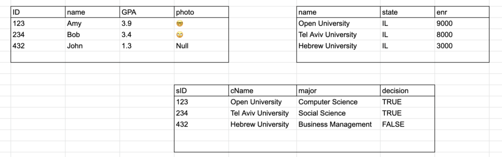
);ow that our tables are set up, let’s insert some data into them. Here are some students you can use:
INSERT INTO Student (
                     sID,
                     name,
                     GPA,
                     photo
                    ) VALUES (
                              123,
                              'Amy',
                              3.9,
                              '🤓'
                             ),
                             (
                              234,
                              'Bob',
                              3.4,
                              '🙄'
                             ),
                             (
                              432,
                              'John',
                              1.3,
                              null
                             );
Now, let’s add some colleges:
INSERT INTO College (
                     name,
                     state,
                     enr
                    ) VALUES (
                              'Open University',
                              'IL',
                              9000
                             ),
                             (
                              'Tel Aviv University',
                              'IL',
                              8000
                             ),
                             (
                              'Hebrew University',
                              'IL',
                              3000
                             );
Finally, let’s populate our Apply relation:
INSERT INTO Apply (
                     sID,
                     cName,
                     major,
                     decision
                    ) VALUES (
                              123,
                              'Open University',
                              'Computer Science',
                              true
                             ),
                             (
                              123,
                              'Tel Aviv University',
                              'Business Management',
                              true
                             ),
                             (
                              234,
                              'Hebrew University',
                              'Social Science',
                              true
                             ),
                             (
                              432,
                              'Hebrew University',
                              'Art',
                              false
                             );
Moving on, let’s explore SQL constraints and the different types of queries we can use to retrieve and manipulate data in our database.
SQL Constraints
In The Relational Model, a database can have constraints, which are rules that must be followed in order to maintain the integrity of the data. These rules ensure the accuracy and reliability of data in a database and can be applied to individual columns or the entire table.
Examples include NOT NULL and DEFAULT constraints, as well as UNIQUE, PRIMARY KEY, FOREIGN KEY, CHECK, and INDEX constraints. These constraints can be specified when the table is first created or added later using the ALTER TABLE statement. In the next post of this series, we will delve deeper into the topic of Constraints and Triggers.
SQL Primary and Foreign Keys
A primary key is a unique attribute or set of attributes used to identify each tuple in a table. For example, the ID attribute might be the primary key for the student table.
A foreign key, on the other hand, is an attribute in one table that refers to the primary key in another table. For example, the College attribute in the student table might be a foreign key that refers to the primary key (name) in the college table.
When we set up our database and tables earlier, we used primary and foreign key constraints. However, it is worth noting that a primary key can still have a null value. To prevent this, we can create the table with the following syntax:
CREATE TABLE Student (
                      ID INT PRIMARY KEY NOT NULL,
                      name TEXT,
                      GPA REAL,
                      photo BLOB
                      );
Basic SQL CRUD Queries
CRUD Queries are essential for interacting with a database. CRUD stands for Create Read Update Delete, and each of these operations corresponds to a different SQL query. Let’s start with the SELECT query, which is used to retrieve data from the database. The basic syntax for a SELECT statement is:
SELECT * FROM table_name;The asterisk (*) is a wildcard that stands for all columns in the table. Alternatively, you can also specify specific columns by listing them separated by commas:
SELECT column_1, column_2, column_3 FROM table_name;To filter the results of your SELECT statement, you can use a WHERE clause. For example, to retrieve all students with a GPA above 3.5, you can use the following query:
SELECT * FROM Student WHERE GPA > 3.5;Logical operators like AND, OR, and NOT can be used to further narrow down your results. For example, to retrieve all students with a GPA above 3.5 and a name starting with the letter ‘A’, you can use the following query:
SELECT * FROM Student WHERE GPA > 3.5 AND name LIKE 'A%';The SELECT statement is composed of three main clauses: SELECT, FROM, and WHERE, and it is the foundation of the SQL language. It corresponds to the projection and selection operations in relational algebra and allows you to retrieve data from your database in a variety of ways.
SELECT A1, A2, ..., An
FROM R1, R2, ..., Rm
WHERE condition
UPDATE
Another useful query is the UPDATE statement, which is used to modify data in a table. The basic syntax for an UPDATE statement is:
UPDATE table_name SET column_1 = value_1 WHERE condition;For example, let’s say we want to update the photo of student 123 to 👱🏽♀️:
UPDATE Student SET photo = '👱🏽♀️' WHERE ID = 123;INSERT
The INSERT statement is used to add new data to a table. Its basic syntax is:
INSERT INTO table_name (column_1, column_2, column_3) VALUES (value_1, value_2, value_3);For example, to add a new student named ‘Alice’ with an ID of 567 and a GPA of 3.7, you can use the following query:
INSERT INTO Student (sID, name, GPA) VALUES (567, 'Alice', 3.7);DELETE
Lastly, we have the DELETE statement, which is used to remove data from a table. The basic syntax for a DELETE statement is:
DELETE FROM table_name WHERE condition;
For example, let’s say we want to delete the student with an ID of 234:
DELETE FROM Student WHERE sID = 234;It’s worth noting that the DELETE statement is irreversible, so make sure to use it carefully and only when necessary.
SQL JOIN Operators
In SQL, a JOIN operator is used to combine rows from two or more tables based on a related column between them.
Going to our SELECT FROM WHERE statement:
SELECT A1, A2, ..., An
FROM R1, R2, ..., Rm
WHERE condition
In our SELECT statement’s FROM clause, we list tables separated by commas, forming an implicit cross-product of those tables. However, it is also possible to have an explicit join of tables, following the style of relational algebra.
There are several types of JOINs in SQL:
INNER JOIN: Returns only the rows that match the join condition in both tables. This is the default type ofJOINif no specificJOINtype is specified.LEFT JOINorLEFT OUTER JOIN: Returns all rows from the left table and the matching rows from the right table. If there is no match,NULLvalues are returned for the right table’s columns.RIGHT JOINorRIGHT OUTER JOIN: Returns all rows from the right table and the matching rows from the left table. If there is no match,NULLvalues are returned for the left table’s columns.FULL OUTER JOIN: Returns all rows from both tables, whether or not there is a match in the other table. If there is no match,NULLvalues are returned for the non-matching columns.
Here is an example of an INNER JOIN in SQL:
SELECT *
FROM table1 INNER JOIN table2
ON table1.column = table2.column;
Note that none of these operators is actually adding expressive power to SQL. All of them can be expressed using other constructs, but they can be quite useful in formulating queries and especially the OUTER JOIN, is fairly complicated to express without the OUTER JOIN operator.
Implicit JOIN Query
To combine columns from two or more tables, you can use a JOIN query in SQL. There are two ways to write a JOIN query: with an implicit JOIN or with an explicit JOIN operator.
Here is an example of an implicit natural JOIN query:
SELECT name,
              major
  FROM Student,
             Apply
 WHERE Student.ID = Apply.sID;
This query will return the student’s name from the Student table and the major from the Apply table, where the condition is that the student ID in the Student table matches the student ID in the Apply table.
But the same query can be written with an explicit JOIN operator as follows:
SELECT name,
       major
  FROM Student
       INNER JOIN Apply
       ON Student.ID = Apply.sID;
The result of this query will be the same as the implicit JOIN query. The difference is that the JOIN and the join condition are specified in the FROM clause instead of the WHERE clause.
Since the default JOIN is inner, we can drop the INNER from the query and we will get the same result:
SELECT name,
       major
  FROM Student
       JOIN Apply
       ON Student.ID = Apply.sID;
Adding DISTINCT
If multiple rows in the result table satisfy the search condition, the result table may contain duplicate rows. To remove duplicates, you can use the DISTINCT keyword in the SELECT clause, like this:
SELECT DISTINCT name,
                                major
                    FROM Student,
                                Apply
 WHERE Student.ID = Apply.sID;
The DISTINCT src * keyword ensures that only unique rows are selected.
As a result, if a selected row duplicates another row in the result table, the duplicate row is ignored (it is not put into the result table).
Otherwise, if you do not include DISTINCT in a SELECT clause, you might find duplicate rows in your result, because SQL returns the column’s value for each row that satisfies the search condition.
Note that NULL values are always treated as duplicate rows for DISTINCT.
INNER JOIN
The explicit JOIN syntax is generally considered to be more readable and more flexible than the implicit JOIN syntax, as it explicitly specifies the type of JOIN to be performed and the join condition in the FROM clause.
In the above queries, we combined students where IDs match the sID of the apply table. The following query, adding a few other attributes while combining the third table:
SELECT sID,
       name,
       GPA,
       major,
       cName,
       enr
  FROM (
           Apply
           JOIN
           Student ON sID = ID
       )
       JOIN
       College ON cName = College.name;
You might have noticed the parentheses around the first JOIN in the FROM clause, this will put organise the query so the college name join is performed on the result of the first join. Without the parentheses, the query will not perform differently, because the order will be executed the same, but it is still not a bad idea to emphasise the order of the query execution by adding parentheses.
NATURAL JOIN
A natural join query in SQL is a type of JOIN query that is based on the common columns between two tables. The common columns are columns that have the same name and data type in both tables.
In a natural join query, the join condition is automatically generated based on the common columns between the two tables. This means that you do not need to specify the join condition explicitly in the ON clause.
Here is an example of a natural join query:
SELECT name,
       major
  FROM Student
       NATURAL JOIN
       Apply;
Additionally, the NATURAL JOIN eliminates duplicate columns that are created. IF we will run the above query with * instead of specifying the columns:
SELECT *
  FROM Student
       NATURAL JOIN
       Apply;
You’ll see that only one ID column is the returned set. You might want to rename the Student.ID to sID which you could use the following query for that.
ALTER TABLE Student RENAME Column 'ID' TO 'sID';The result will look like this:
As you can see, there’s only one column named sID.
And we’ll run this query without the NATURAL JOIN such as:
SELECT DISTINCT sID
  FROM Student,
       Apply;
We will get the following error: “ambiguous column name: sID”.
The USING clause
Now there’s a feature that goes along with the join operator in SQL that’s considered actually better practice than using the NATURAL JOIN and it’s called the USING clause.
And the USING clause explicitly lists the attributes that should be equated across the two relations. So, we’re going to take away the natural here, we’re just going to use the regular inner join, but then we’re going to specify that the student ID is the attribute that should be equated across Student and Apply:
SELECT *
  FROM Student
       JOIN
       Apply USING (
           sID
       );
Or just to make it more interesting, let’s add some conditions:
SELECT name,
       GPA
  FROM Student
       JOIN
       Apply USING (
           sID
       )
 WHERE major = 'Computer Science' AND
       cName = 'Open University';
The reason this is considered better practice, to make this explicit, is that the natural join implicitly combines columns that have the same name.
It’s possible, say, to add a column to a relation that has the same name as the other relation, or not realize that two relations have the same column name. And the system will sort of underneath the covers, equate those values.
Whereas, when we put the attribute name in the query we’re saying explicitly that this attribute does mean the same thing across the two relations.
Self-JOIN with USING
Let’s find all the students that have the same GPA:
SELECT S1.sID,
       S1.name,
       S1.GPA,
       S2.sID,
       S2.name,
       S2.GPA
  FROM Student S1
       JOIN
       Student S2 USING (
           GPA
       )
 WHERE S1.sID < S2.sID;
Note that if we’ll put the condition in an ON clause, we will get a syntax error.
Back to our natural join, if we’ll run a NATURAL JOIN as a self-join query such as:
SELECT *
  FROM Student S1
       NATURAL JOIN
       Student S2;
We will get all the records of students that have no null values since null is considered a duplicate, and S2 columns are eliminated by the natural join.
OUTER JOIN
We’ve seen different types of JOIN operators, such as INNER JOIN, NATURAL JOIN, and INNER JOIN with the USING clause. Let’s look at another type of JOIN operator, the OUTER JOIN.
For example, consider the following INNER JOIN query:
SELECT name,
       sID,
       cName,
       major
  FROM Student
       INNER JOIN
       Apply USING (
           sID
       );
This query returns the columns specified in the SELECT clause for all the students who have applied somewhere. However, suppose we want to also get all the students who did not apply.
One way to do this is to use a LEFT OUTER JOIN, like this::
SELECT name,
       sID,
       cName,
       major
  FROM Student
       LEFT OUTER JOIN
       Apply USING (
           sID
       );
The following is a revised version of the paragraph:
“We’ve seen different types of JOIN operators, such as INNER JOIN, NATURAL JOIN, and INNER JOIN with the USING clause. Let’s look at another type of JOIN operator, the OUTER JOIN.
For example, consider the following INNER JOIN query:
SELECT name, sID, cName, major
FROM Student INNER JOIN Apply USING (sID);
This query returns the columns specified in the SELECT clause for all the students who have applied somewhere. However, suppose we want to also get all the students who did not apply.
One way to do this is to use a LEFT OUTER JOIN, like this:
SELECT name,
       sID,
       cName,
       major
  FROM Student
       LEFT OUTER JOIN
       Apply USING (
           sID
       );
This query returns more tuples, including those that have NULL values for the cName and major columns. These tuples represent students who did not apply and therefore have no corresponding rows in the Apply table.
By the way, the tuples with blank/null values are usually referred to as “dangling tuple”.
Implicit OUTER
As with the inner join, we can actually abbreviate this. When we have left or, as we’ll see, right,
or full, we can take a word, away the word outer and that will implicitly do the left outer join:
SELECT name,
       sID,
       cName,
       major
  FROM Student
       LEFT JOIN
       Apply USING (
           sID
       );
Run this and we get, again, the same result. Just an abbreviation.
SQL NATURAL LEFT JOIN
A NATURAL OUTER JOIN in SQL is a type of join that combines rows from two tables based on the common columns between them, similar to a NATURAL INNER JOIN. However, unlike an INNER JOIN, which only returns the rows that have a match in both tables, a NATURAL OUTER JOIN will also return all the rows from one of the tables, even if there is no match in the other table. This is achieved by using the OUTER JOIN keyword and specifying either a LEFT, RIGHT, or FULL join.
LEFT JOIN: Returns all rows from the left table (Student in the example below), and any matching rows from the right table (Apply). If there is no match, NULL values will be displayed for the right table’s columns.
RIGHT JOIN: Similar to a LEFT JOIN, but returns all rows from the right table (Apply) and any matching rows from the left table (Student).
FULL JOIN: Returns all rows from both tables, regardless of whether there is a match in the other table. If there is no match, NULL values will be displayed for the missing columns.
Here is an example of a NATURAL OUTER JOIN in SQL:
SELECT name,
       sID,
       cName,
       major
  FROM Student
       NATURAL LEFT OUTER JOIN
       Apply;
It’s worth noting that the USING clause, which specifies the common columns between the two tables, is often omitted in NATURAL OUTER JOINs. However, this is not necessarily the best software engineering practice and should be used with caution.
NATURAL OUTER JOINS are useful when you want to include all rows from both tables in the result set, even if there is no matching data. This can be useful, for example, when you want to see a complete list of all students and their corresponding application data.
Implicit NATURAL LEFT JOIN
All the JOIN operations discussed so far can be rewritten using regular SQL without JOIN operators. This is relatively straightforward for INNER JOIN and NATURAL JOIN, as they can be expressed using SELECT, FROM, and WHERE clauses with cross products and conditions. However, it may not be as obvious that the OUTER JOIN can also be expressed using regular SQL. Nonetheless, it is possible to rewrite the OUTER JOIN without using the OUTER JOIN keyword. And here it is:
SELECT name,
       Student.sID,
       cName,
       major
  FROM Student,
       Apply
 WHERE Student.sID = Apply.sID
UNION
SELECT name,
       sID,
       NULL,
       NULL
  FROM Student
 WHERE sID NOT IN (
           SELECT sID
             FROM Apply
       );
This rewritten query effectively performs the same operation as a NATURAL OUTER JOIN, which combines rows from two tables based on common columns and eliminates duplicate columns, and returns all rows from one table and any matching rows from the other table.
In this rewritten query, the first SELECT statement uses a WHERE clause to select all the rows from the Student and Apply tables that match based on the sID column. The second SELECT statement uses a WHERE clause with a NOT IN subquery to select all the rows from the Student table where the sID does not appear in the Apply table. These two SELECT statements are combined using a UNION operator to create the final result set.
Overall, this rewritten query is a good example of how the OUTER JOIN operation can be expressed using regular SQL without using any JOIN operators. It is concise, easy to understand, and effectively performs the same operation as the NATURAL OUTER JOIN query.
NATURAL RIGHT OUTER JOIN
In our query, we retained all student tuples whether or not they matched an apply tuple. What if we wanted to do things the other way around? What if we wanted to retain apply tuples whether or not they matched a student tuple?
Well, you can probably guess that all we need to do is swap the order of apply and student and put apply on the left instead.
It so happens that our database actually doesn’t have any apply tuples that don’t match, so we’ll add those tuples right now.
INSERT INTO Apply VALUES (
                      569,
                      'Hebrew Univesity',
                      'Psychology',
                      1
                  ),
                  (
                      569,
                      'Hebrew Univesity',
                      'Law',
                      1
                  );
We’ve added a student 569 applying to Hebrew University for a couple of majors and we don’t have a matching 569 in our student table. So going back to the original query and swapping the order so that we keep all tuples that apply whether or not they match.
Let’s go ahead and run the query:
SELECT name,
       sID,
       cName,
       major
  FROM Apply
       NATURAL LEFT OUTER JOIN
       Student;
And we take a look down here and we see that we have those two applications of 569 even though there’s no matching student name.
Now not surprisingly SQL actually has a companion to the left outer join called the right outer join. So I don’t actually have to swap my relations, I can actually use the right outer join with apply on the right-hand side.
And what this says is we’re going to find the student tuples that match the apply tuples, and then if there are tuples in apply that don’t match the students, we’ll add those padded with nulls.
So here goes:
SELECT name,
       sID,
       cName,
       major
  FROM Student
       NATURAL RIGHT OUTER JOIN
       Apply;
Again, we’re getting the same result.
FULL OUTER JOIN
Now I’m sure what you’re thinking is what if we want to have unmatched tuples from both the left and the right appear in our result. And that’s what’s called the full outer join. So let’s just change this right now to the full outer join.
SELECT name,
       sID,
       cName,
       major
  FROM Student
       NATURAL FULL OUTER JOIN
       Apply;
And let’s move back to using the USING clause which I like better, like that.
SELECT name,
       sID,
       cName,
       major
  FROM Student
       FULL OUTER JOIN
       Apply USING (
           sID
       );
And let’s go ahead and run the query and now we see that we have the unmatched apply tuples with null values for the name and we also have the unmatched student tuples. With null values for the college name and major.
Not surprisingly the full outer join can be expressed in other ways. We’re going to start by expressing the full outer joinusing a combination of the left and right outer join.
So, here we go:
       major
  FROM Student
       LEFT OUTER JOIN
       Apply USING (
           sID
       )
UNION
SELECT name,
       sID,
       cName,
       major
  FROM Student
       RIGHT OUTER JOIN
       Apply USING (
           sID
       );
Remember that the UNION operator automatically eliminates duplicates, so in the end we will get the same result.
We can also simulate without using any join operator:
SELECT name,
       Student.sID,
       cName,
       major
  FROM Student,
       Apply
 WHERE Student.sID = Apply.sID
UNION
SELECT name,
       sID,
       NULL,
       NULL
  FROM Student
 WHERE sID NOT IN (
           SELECT sID
             FROM Apply
       )
UNION
SELECT NULL,
       sID,
       cName,
       major
  FROM Apply
 WHERE sID NOT IN (
           SELECT sID
             FROM Student
       );
The first part finds all of the matching student and apply records. The second part adds to that those students who aren’t present in apply. So it gives us their name and ID and the two null values for the attributes from the apply relation. And then the third part finds those apply records where there’s not a matching student, and so it gives us the three attributes from apply, but then gives us a null for student name.
SQL Null Values
Again, the SQL NULL is a special value that represents a missing or unknown value in a database table. It is important to note that a NULL value is not the same as a zero value or a field that contains spaces.
Therefore, a field with a NULL value has no value at all, and it appears (conceptually) as a blank space in the table.
Hence, it is important to understand the distinction between NULL values and other types of values, as this can affect the results of database queries and the integrity of the data.
Indeed, when working with databases, it is essential to consider the possibility of NULL values and to handle them appropriately. If a value can never be null, meaning the record will be useless without the value being defined, we could use a constraint to prevent the insertion of null values for the said attribute.
To illustrate a query involving Null Values, let us suppose that the semester is approaching and we need to ask all students to submit their GPA data. We can execute the query below to achieve this:
SELECT name
FROM Student
WHERE GPA IS NULL;
This query will return all students that have not yet provided their GPA. We can then use this information to send out emails to the students reminding them of the requirement.
SQL Nested Subqueries
SQL nested subqueries are subqueries that are placed within another SQL query. They are used to return data that is used in the main query as a condition to further restrict the data to be retrieved. Nested subqueries can be used in the SELECT, WHERE, and FROM clauses. As well as in INSERT, UPDATE and other operators, but for now let’s start looking at subqueries in the WHERE clause.
Subqueries in the WHERE clause
So let’s launch right into our first query shows a sub-query in the where clause:
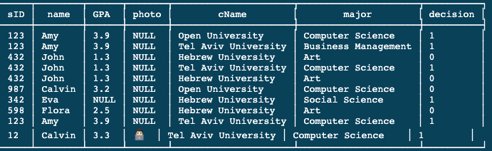
 SELECT sID, name
 FROM Student
 WHERE ID in (SELECT sID FROM Apply WHERE major = 'Computer Science');
This query finds the IDs and names of all students who have applied to major in computer science at some college.
The subquery in the WHERE clause namely:
SELECT sID FROM Apply WHERE major = 'Computer Science';Selects all student IDs who have applied to major in computer science from the apply table. Now that we have that set of IDs our outer query, namely:
 SELECT sID, name
 FROM Student
 WHERE ID in ...;
Says, let’s take all the names and IDs from our Student relation, where the ID of the Student relation is in that set of sID‘s returned from our inner query.
But we can actually do this query without the inner subquery similar to what we did a few lines above in the basic JOIN query:
SELECT sID, name
FROM Student, Apply
WHERE Student.ID = Apply.sID and major = 'Computer Science';
But in that query, if you have a student that applied to computer science in two different colleges, you will get that student twice, whereas the nested subquery will match the student ID against the set of IDs that comes from the inner query.
Of course, this can be easily fixed by using DISTINCT:
SELECT DISTINCT sID, name
FROM Student, Apply
WHERE Student.ID = Apply.sID and major = 'Computer Science';
Why do we need nested sub-queries
At this point, we might ask ourselves what’s the point of a subquery if we can get the same result with a simple JOIN query. To understand that, let’s look at another example:
For demonstrating this example, let me share my current DB tables:
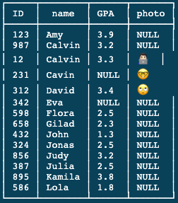
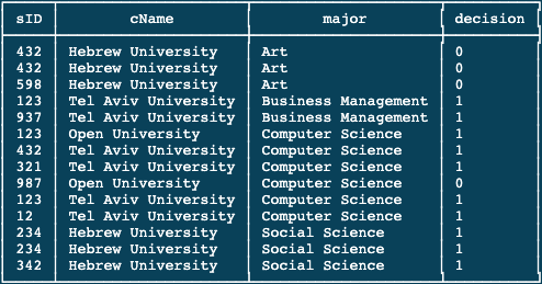
SELECT name
FROM Student
WHERE ID in (SELECT sID FROM Apply WHERE major = 'Computer Science');
Having that setup, the query returns as follows:

If we would run this query by joining the two tables:
SELECT name
FROM Student, Apply
WHERE ID = sID and major = 'Computer Science';
As a result, we get this:
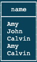
Because we get two copies when a student has applied to major in computer science in two different places. So let’s add a DISTINCT to our query:
SELECT DISTINCT name
FROM Student, Apply
WHERE ID = sID and major = 'Computer Science';
But then we get only one Calvin even though there are two different Clavins that applied to CS.
Why Duplicates Matter
Well, imagine we want to compute the average GPA of the students who have applied to CS:
SELECT GPA
FROM Student
WHERE ID in (SELECT sID FROM Apply WHERE major = 'Computer Science');
The above query will give us the correct list of GPAs, but if we’ll have two students who applied to CS with the same GPA and we run the following query:
SELECT DISTINCT GPA
FROM Student, Apply
WHERE ID = sID and major = 'Computer Science';
As a result, we will get the wrong list of GPAs to compute the average from. The only way to compute the correct average is to use the version of the query where we have the sub-query in the WHERE clause.
Last but not least, let’s write a query to find all students that applied to computer science but did not apply to social science:
SELECT sID, name
FROM Student
WHERE EXISTS (SELECT sID FROM Apply WHERE major = 'Computer Science')
AND NOT EXISTS (SELECT sID FROM Apply WHERE major = 'Social Science');
But for now, let’s move to subqueries in the FROM and SELECT clauses.
Nested Subqueries in SELECT
In the above section, we looked into nested subqueries in the WHERE clause – in the condition. If we use a sub-query in the SELECT, then what we’re doing is writing a SELECT expression, a sub-select expression, that produces the value that comes out of the query.
SELECT DISTINCT College.name,
                state,
                GPA
  FROM College,
       Apply,
       Student
 WHERE College.name = Apply.cName AND
       Apply.sID = Student.ID AND
       GPA >= (
                  SELECT MAX(GPA)
                    FROM Student,
                         Apply
                   WHERE Student.ID = Apply.sID AND
                         Apply.cName = College.name
              );
So, as this query might look a little bit complex, let’s start explaining it with the expected result. Run this query, you will get a 3-column relation as a result with the college name, the college state, and the highest GPA of the students who applied to this college.
The inner query provides us with the highest GPA of a student who has applied to the college, using the max aggregate function, which we will see later, and a JOIN query of Student and Apply relations. Then the outer query asks for the college name, the college state and the student GPA, compared to the highest GPA the inner query found.
Essentially, with a little modification, we can do the same with nesting the sub-query in the SELECT clause:
SELECT DISTINCT College.name,
                state,
                (
                    SELECT DISTINCT GPA
                      FROM Apply,
                           Student
                     WHERE College.name = Apply.cName AND
                           Apply.sID = Student.ID AND
                           GPA >= (
                                      SELECT MAX(GPA)
                                        FROM Student,
                                             Apply
                                       WHERE Student.ID = Apply.sID AND
                                             Apply.cName = College.name
                                  )
                )
                AS GPA
  FROM College;
Which will return the same result.
Now, there is much more to explore with nested subqueries in the WHERE clause, but this should already give us an idea of what they look like.
Table Variables
Having already learned some basics of the SQL language, let us dive deeper into more features. Specifically – table variables and set operators.
In particular, table variables, serve two purposes – to make the query more readable and to rename relations in the FROM clause when two instances of the same relation are used.
To demonstrate it, let’s begin with a large join query that will emphasise how to incorporate table variables. This query incorporates all three relations, joining them on their shared attributes and then selecting a variety of information.
Variables in the SELECT Clause
Though the result of this query can be seen below, however, the main purpose of the query is to show how table variables are used in the FROM clause.
SELECT Student.ID AS sID, Student.name AS sName, GPA, Apply.cName, enr
FROM Student, College, Apply
WHERE Apply.sID = sID and Apply.cName = College.name;
As a result, you should get something as follows:
However, the result is not what we are interested in, rather we want to understand the table variables.
Variables in the FROM Clause
Similar to what we did in the SELECT clause with the AS keyword, we can do on the FROM clause without it.
SELECT S.ID AS sID, S.name AS sName, GPA, A.cName, enr
FROM Student S, College C, Apply A
WHERE A.sID = sID and A.cName = C.name;
In this case, we’re not changing the outcome of the query, we’re really just making it a bit more readable. Having that said, we’ll run now the query and we’ll get the same result. But the query looks much better, isn’t it?
Another example of FROM variables that will make even more sense would be as follows:
SELECT S1.sID, S1.name AS sName, S1.GPA, S2.name as sName, S2.GPA
FROM Student S1, Student S2
WHERE S1.GPA = S2.GPA;
As you can imagine, this query is supposed to find all students that have the same GPA. However, if you’ll run this query, you might find out that it returns also the same student as S1 and S2.
In that case, we can add another condition to the WHERE clause:
SELECT S1.sID, S1.name AS sName, S1.GPA, S2.name as sName, S2.GPA
FROM Student S1, Student S2
WHERE S1.GPA = S2.GPA and S1.ID <> S2.ID;
While this will get us rid of listing the same students side by side, we still have a repetition of one-time S1 vs S2 and then S2 vs S1.
To that end, there is only one little thing we can change in our query to avoid it:
SELECT S1.sID, S1.name AS sName, S1.GPA, S2.name as sName, S2.GPA
FROM Student S1, Student S2
WHERE S1.GPA = S2.GPA and S1.ID < S2.ID;
Finally, we now have a result where all lines in our table are unique. Which is probably the answer we wanted in the first place.
Set Operators
Next, let’s take a look at the set operators, starting with the union operator:
The Union Operator
SELECT name FROM College
UNION
SELECT name FROM Student;
Upon running this query, we’ll get all names of students and colleges listed in one column. More than that, if we would have done it as follow:
SELECT name AS cName FROM College
UNION
SELECT name AS sName FROM Student;
As a result, we would have got an even more confusing column, since UNION will put all the names of colleges and students under the column named cName.
Additionally, the result is sorted. Moreover, the union operator in SQL eliminates duplicates by default in its results. For example, if there are two Amys, only one Amy will be in the result. Similarly, two Bob’s will become one in the result. The system used today, SQLite, eliminates duplicates by sorting the result.
Having that said, other Relational Databases might behave differently with the UNION operator.
For this reason, it is important to note that one cannot rely on the same query yielding the same results when executed on different systems, or even on the same system at a different time.
The ORDER BY Operator
Thus the UNION operator listed all the names of students and colleges, there might be cases where we will want the names to be sorted first by their type i.e. college and then by alphabetic order.
To do so, we can run the following:
SELECT name FROM College
UNION ALL
SELECT name FROM Student;
But what if we want to ensure the order is done by name no matter if it’s a college or a student?
For this, we can add the ORDER BY operator to our query:
SELECT name AS cName FROM College
UNION ALL
SELECT name AS sName FROM Student
ORDER BY name;
Unless you don’t mind the order of the result, ORDER BY is always a good idea.
The INTERSECT Operator
Let’s say we want to find all students applying for both, computer science and business management, we can do that by using the INTERSECT operator.
SELECT sID FROM Apply WHERE major = 'Computer Science'
INTERSECT
SELECT sID FROM Apply WHERE major = 'Business Management';
Another way to do it is as follows:
SELECT A1.sID
FROM Apply A1, Apply A2
WHERE
      A1.sID = A2.sID
      AND
      A1.major = 'Computer Science'
      AND
      A2.major = 'Business Management';
As a result, we might get some duplications of the same sID, but that’s easy to get rid of:
SELECT DISTINCT A1.sID
FROM Apply A1, Apply A2
WHERE
      A1.sID = A2.sID
      AND
      A1.major = 'Computer Science'
      AND
      A2.major = 'Business Management';
And that will get rid of all duplicates.
The EXCEPT Operator
Instead of getting all students who applied to both majors, we’re now getting students that applied only to one of the majors.
SELECT sID FROM Apply WHERE major = 'Computer Science'
EXCEPT
SELECT sID FROM Apply WHERE major = 'Business Management';
Since some database systems don’t support the EXCEPT operator, we can run this query as follows:
SELECT A1.sID
FROM Apply A1, Apply A2
WHERE
      A1.sID = A2.sID
      AND
      A1.major = 'Computer Science'
      AND
      A2.major <> 'Business Management';
But if you have enough records on your database, you’ll find out that this query is not as precise as EXCEPT. Since the same student that applied to these both majors, could apply to other ones, this last query cannot filter all students that applied only to one of these majors.
Aggregate Functions
Aggregate functions are functions that take a collection (a set or multiset) of values
as input and return a single value. SQL offers five built-in aggregate functions:
- Average: avg
- Minimum: min
- Maximum: max
- Total: sum
- Count: count
The input to sum and avg must be a collection of numbers, but the other operators can operate on collections of non-numeric data types, such as strings, as well.
These are functions that will appear in the SELECT clause initially and they perform computations over sets of values in multiple rows of a relation.
HAVING and GROUP BY
Once we introduced the aggregation functions, we can also add two classes to the SQL SELECT from where statement, the GROUP BY and HAVING clause.
The GROUP BY allows us to partition our relations into groups, and then will compute aggregate functions over each group independently. The HAVING condition allows us to test filters on the results of aggregate values, whereas the WHERE clause applies to single rows at a time.
SELECT avg(GPA)
FROM Student;
As you can imagine, this query will return the average GPA of all students in the Student table.
Our second query is a bit more complicated. It involves a join.
SELECT min(GPA)
  FROM Student,
       Apply
 WHERE Student.sID = Apply.sID AND
       major = 'Computer Science';
This query finds the minimum GPA of students who have applied for a CS major.
To see the result without aggregation we can run the query without the aggregation function:
SELECT GPA
  FROM Student,
       Apply
 WHERE Student.sID = Apply.sID AND
       major = 'Computer Science';
Now when we run the aggregation function, it should be clearer that it’s finding the lower GPA of students who have applied to CS.
The Count Function
So far we’ve seen the avg and min functions. This query shows the count function:
SELECT count(*)
  FROM Student
 WHERE GPA > 2.5;
And it returns the number of students with GPA greater than 2.5.
Similarly, the following query returns the number of applications to Tel Aviv University:
SELECT count(*)
  FROM Apply
 WHERE cName = 'Tel Aviv University';
But this query has a similar issue to what we looked at previously, it counts all the rows of students who applied to Tel Aviv University, even those who applied multiple times. To fix that we can run it as follows:
SELECT count(DISTINCT sID)
  FROM Apply
 WHERE cName = 'Tel Aviv University';
Aggregation with Nest Subqueries
But this query is probably not written correctly because let’s say we want to get the average GPA of students that applied to CS, we will get the wrong average. To understand why run the following query:
SELECT *
  FROM Student,
       Apply
 WHERE Student.sID = Apply.sID AND
       major = 'Computer Science';
You can see that some rows are duplicated, to fix it we can rewrite the query using a nested subquery:
SELECT *
  FROM Student
 WHERE sID IN (
           SELECT sID
             FROM Apply
            WHERE major = 'Computer Science'
       );
Now that we don’t get these duplicated rows we can run it with the avg function and it will correctly count students’ GPA only one time:
SELECT avg(GPA)
  FROM Student
 WHERE sID IN (
           SELECT sID
             FROM Apply
            WHERE major = 'Computer Science'
       );
The following query finds the amount by which the average GPA of students who apply to computer science exceeds the average of students who don’t apply to computer science:
SELECT CS.avgGPA - NonCS.avgGPA
  FROM (
           SELECT avg(GPA) AS avgGPA
             FROM Student
            WHERE sID IN (
                      SELECT sID
                        FROM Apply
                       WHERE major = 'Computer Science'
                  )
       )
       AS CS,
       (
           SELECT avg(GPA) AS avgGPA
             FROM Student
            WHERE sID NOT IN (
                      SELECT sID
                        FROM Apply
                       WHERE major = 'Computer Science'
                  )
       )
       AS nonCS;
So we’re using subqueries in the FROM clause, which allows us to write a select from where expression, and then use the result of that expression as if it were an actual table in the database. As we saw in a few sections above, if a nested query returns a single value, we can add it to the select clause:
SELECT DISTINCT (
                    SELECT avg(GPA) AS avgGPA
                      FROM Student
                     WHERE sID IN (
                               SELECT sID
                                 FROM Apply
                                WHERE major = 'Computer Science'
                           )
                )
-               (
                    SELECT avg(GPA) AS avgGPA
                      FROM Student
                     WHERE sID NOT IN (
                               SELECT sID
                                 FROM Apply
                                WHERE major = 'Computer Science'
                           )
                )
  FROM Student;
And we’ll get the same result.
The Group By Clause
The GROUP BY clause is only used in conjunction with aggregation, to demonstrate it, let’s start with a simple query:
ELECT cName,
       count(*)
  FROM Apply
 GROUP BY cName;
This query finds the number of applications for each college. And it’s doing so by using grouping. Effectively what grouping does, is it takes a relation and it partitions it by values of a given attribute or set of attributes.
Specifically in this query, we were taking the apply relation and we broke into groups where each group has one of the college names, and then for each group, we returned one tuple in the result containing the college name for that group and the number of tuples in the group.
To illustrate what this query does, we can run the following query:
SELECT *
  FROM Apply
 ORDER BY cName;
And see the number of lines for each college.
Group by with JOIN
Here is a more complicated group by query:
SELECT cName,
       major,
       min(GPA),
       max(GPA)
  FROM Student,
       Apply
 WHERE Student.sID = Apply.sID
 GROUP BY cName,
          major;
In this case, we’re grouping by two attributes, we also have a join involved and we’re computing two aggregate functions in our result. As a result, we’re getting for college and major combination the minimum and maximum GPAs for the students who’ve applied to that college.
The following group by query will find the number of colleges each of our students applied to:
SELECT Student.sID,
       name,
       count(DISTINCT cName)
  FROM Student,
       Apply
 WHERE Student.sID = Apply.sID
 GROUP BY Student.sID;
While this query allows us to print the student’s name although it’s not what aggregating here. if will try to print the college name, we’ll get strange behaviour:
SELECT Student.sID,
       name,
       count(DISTINCT cName),
       cName
  FROM Student,
       Apply
 WHERE Student.sID = Apply.sID
 GROUP BY Student.sID;
It prints a random college name from the list of colleges the student applied to. Note that some database systems will throw an error for such queries.
Back to our query, let’s say we want to add all the students who didn’t apply to any college with 0 next to their IDs, we can do that as follows:
SELECT Student.sID,
       count(DISTINCT cName)
  FROM Student,
       Apply
 WHERE Student.sID = Apply.sID
 GROUP BY Student.sID
UNION
SELECT sID,
       0
  FROM Student
 WHERE sID NOT IN (
           SELECT sID
             FROM Apply
       );
And here you get all the student IDs, with those who didn’t apply too.
The HAVING Clause
The HAVING clause applied after the GROUP BY clause and it allows us to check conditions that involve the entire group. In contrast the WHERE clause, it applies to one tuple at a time.
The following query finds colleges that have fewer than five applicants:
SELECT cName
  FROM Apply
 GROUP BY cName
HAVING count( * ) < 5;
So it looks at the apply relation, and it groups it by the college name, so each college has only one tuple, and then we keep only the colleges that have fewer than 5 applicants.
Having that said, it does happen actually that every query that can be written with the GROUP BY and a HAVING clause can be written in another form. In our example it will be as follows:
SELECT DISTINCT cName
  FROM Apply A1
 WHERE 5 > (
               SELECT count( * )
                 FROM Apply A2
                WHERE A2.cName = A1.cName
           );
But sometimes it can be extremely contoured.
Back to our query, with a simple modification, we can include in our result all the colleges that might have more than five applications but less than five applicants:
SELECT cName
  FROM Apply
 GROUP BY cName
HAVING count(DISTINCT sID) < 5;
To close this post with a simple exercise, you explain the following query in the comments:
SELECT major
  FROM Student,
       Apply
 WHERE Student.sID = Apply.sID
 GROUP BY major
HAVING max(GPA) < (
                      SELECT avg(GPA)
                        FROM Student
                  );
Wrapping up
To sum up, the Structured Query Language, or SQL, is a programming language used to manage data stored in a relational database management system (RDBMS). SQL allows users to access and manipulate data stored in databases by writing queries.
On the other hand, SQL is not a programming language and does not have the ability to control flow or define variables like a traditional programming language.
yet, it is a programming language to manage data stored in an RDBMS and allows users to access and manipulate data by writing queries.
We use SQL queries to ask the database questions, retrieve and manipulate data, and perform other operations such as inserting, updating, and deleting data.