An algorithm is a step by step process that describes how to solve a problem in a way that always gives a correct answer. Most problems can be solved by more than one algorithm, but the best algorithm would typically be the one that solves the problem the fastest.
As software developers, we are using algorithms constantly, be it a built-in language function or a completely new algorithm unique to our software. Understanding algorithms is essential for making the right decisions about which algorithms to use and how to make new algorithms that are correct and efficient.
In the following post I want to examine:
The Building Blocks of Algorithms
Informally, an algorithm is any well-defined computational procedure that takes some value as input and produces some value as output. Algorithms have three basic building blocks: sequencing, selection and iteration.
Sequencing – It is crucial to sequence the steps of an algorithm, so the relationship between a given input to the produced output remains correct.
Selection – It is useful to determine a different set of steps in an algorithm by a boolean expression.
Iteration – To produce the desired output, an algorithm often needs to repeat certain steps a certain number of times.
Linear search
To demonstrate these building blocks we could think of a linear search algorithm:
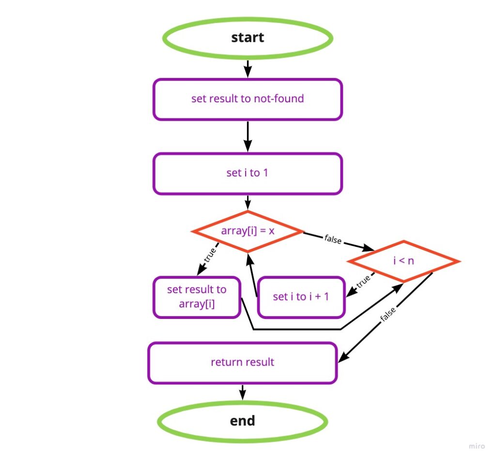
procedure linearSearch(array, n, x)
1. result = not-found
2. for each index i, going from 1 to n, in order:
   A. if array[i] = x, then result = array[i]
3. return result
In the above pseudo-code, we have the linearSearch procedure that takes an array of numbers – array, the number of elements in the array – n, and an element to search in the array – x.
In addition to the parameters array, n and x. The linearSearch procedure uses a variable named result. The procedure assigns an initial value of not-found to result in step 1. Step 2 checks each array element array[1] through array[n] to see if the element contains the value x. Whenever element array[i] equals x, step 2A assigns the current value of array[i] to the result.
The steps of the linearSearch procedure are what we call sequencing, every time we call this procedure it goes through the steps from 1 to 3.
Step 2 is what we call iteration, each element in the array from position 1 to position n goes through step A2.
Step A2 is what we call selection, we check whether the value of array[i] is equal to the searched element x or not.
Categorizing run time efficiency
When a procedure takes too long to solve a problem, it means the software that runs it needs more resources than if the procedure would take shorter to solve this problem. More resources mean a more expensive computer that runs the software.
Big O time is the language and metric we use to describe the efficiency of algorithms. Not understanding it thoroughly can hurt the ability to develop an algorithm.
Time Complexity
The run time of an algorithm would be categorized according to how the number of steps increases as the input size increases. When an algorithm T(n) is bounded by a value that does not depend on the size of the input, it is said to be constant time (aka O(1)). An algorithm is said to be exponential time if T(n) is upper bounded by 2poly(n) where poly(n) is a polynomial in n.
Most algorithms’ run times are somewhere between constant time and exponential time. Let’s explore common run time categories.
Constant time
An algorithm that runs in constant time means that it always takes a fixed number of steps to produce a result, no matter how large the input size increases. T(n) = O(1).
We can demonstrate a constant time algorithm as follows:
procedure findSmallestElementInSortedArray(numbers)
1. return numbers[1] ThefindSmallestElementInSortedArray procedure takes an argument named numbers which is an array of numbers sorted ascendingly, and returns the first element in the numbers array. It doesn’t matter how many elements are in the numbers array, as it assumes the first element is always the smallest one, the operation will always require only one step.
| Number of elements | Number of steps |
| 1 | 1 |
| 10 | 1 |
| 100 | 1 |
| 1000 | 1 |
| 10000 | 1 |
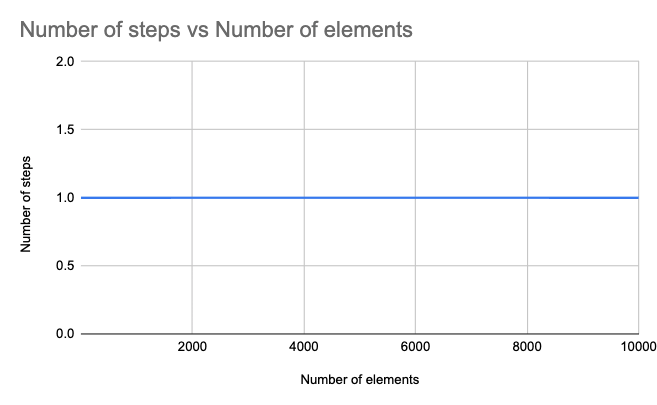
A constant run time is ideal, but in most cases, an algorithm can’t process and produce the desired result in a constant run time.
Logarithmic time
An algorithm that runs in logarithmic time would increase in proportion to the logarithm of the input size. T(n) = O(log n). To demonstrate a logarithmic time algorithm we can use the binary search algorithm.
Binary search
Here is the procedure for binary search:
procedure binarySearch(array, n, x)
1. p = 1, r = n
2. while p ≤ r, do:
    A. q = (p + r) / 2
    B. if array[q] = x then return array[q]
    C. else if array[q] > x, then r = q - 1
    D. else p = q + 1
3. return not-found
This algorithm assumes that the array of numbers is sorted ascendingly. The loop in step 2 look at several elements in the array, but it does not look at every element in the array. Specifically, it looks at log2 n elements, where n is the number of elements in the array.
Let’s visit the binary search run time using a table.
| Number of elements | Number of steps |
| 1 | 1 |
| 10 | 4 |
| 100 | 7 |
| 1000 | 10 |
| 10000 | 14 |
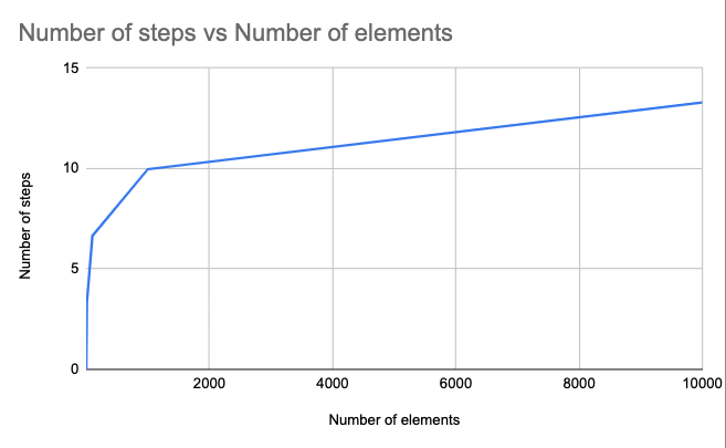
As we see in the graph and table, the number of steps is increasing as the input size increases, but the proportional rate is small.
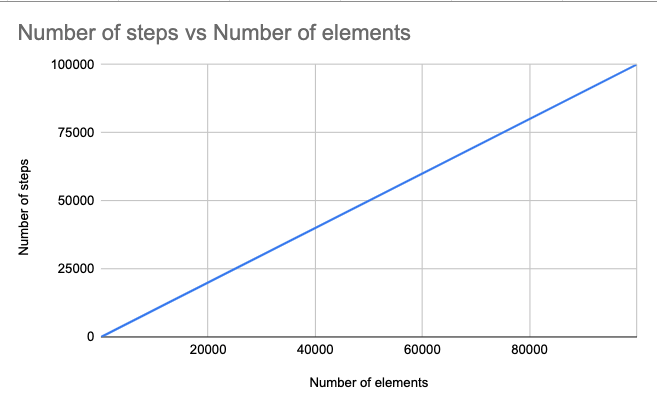
Linear time
An algorithm is said to take linear time when at most, the number of steps it has to do is in direct proportion to the input size. T(n) = O(n). Previously, we looked at the aptly-named linear search procedure that iterates all the elements in the input array and then returns either the found element or not-found. We can do better:
Better linear search
Once the linearSearch procedure went through all the elements, it returns the result. This is not the best way to do a linearSearch, since our procedure is continuing to iterate over the elements in the array even if it found the searched element. A more efficient way to do a linear search would be as follows:
procedure betterLinearSearch(array, n, x)
1. for i = 1 to n:
    A. if array[i] = x, then return array[i]
2. return not-found
As we can see in the Linear search flow chart the value will only return when i is not smaller than n, otherwise, it keeps running the steps 2 and A2, wherein the betterLinearSearch procedure, once the procedure found x it immediately halts with the value, and only if x is not in the array, the procedure keeps iterating the array elements until it reached array[n] and then return not-found.
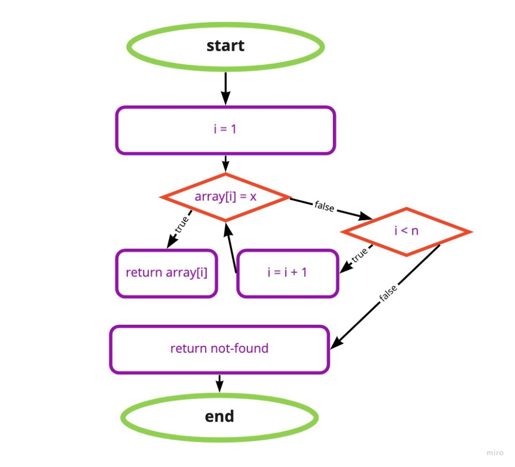
Although in many cases, the number of steps that ourbetterLinearSearch procedure takes is shorter than the number of elements in the array, it will still be considered as linear time, sinceat most, let’s say if x does not exist in the array, the number of steps our algorithm needs to take is the number of elements in the array.
| Number of elements | Number of steps |
| 1 | 1 |
| 10 | 10 |
| 100 | 100 |
| 1000 | 1000 |
Linear time is not ideal, but in some cases, for example, when searching an element in an unsorted array, a linear search is the fastest way to find it.
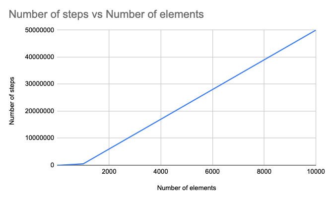
Quadratic time
When an algorithm’s steps increment is directly proportional to the squared size of the input, T(n) = O(n2), its run time complexity is quadratic time.
A sorting algorithm is an algorithm for rearranging the elements of the array – aka permuting the array – so that each element is less than or equal to its successor. For demonstrating the quadratic time complexity, we could use the selection sort algorithm:
Selection sort
Given a list, take the current element and exchange it with the smallest element on the right-hand side of the current element.
Source
Let’s visit the selection sort algorithm pseudo-code:
procedure selectionSort(array, n)
1. for i = 1 to n -1:
    A. smallest = i
    B. for j = i + 1 to n:
        i. if array[j] < array[smallest], then smallest = j
    C. swap array[i] with array[smallest]
Finding the smallest element in array[i…n] is a variant of linear search. First, declare array[i] to be the smallest element seen in the subarray so far, and then go through the rest of the subarray, updating the index of the smallest element every time we find an element smaller than the current smallest.
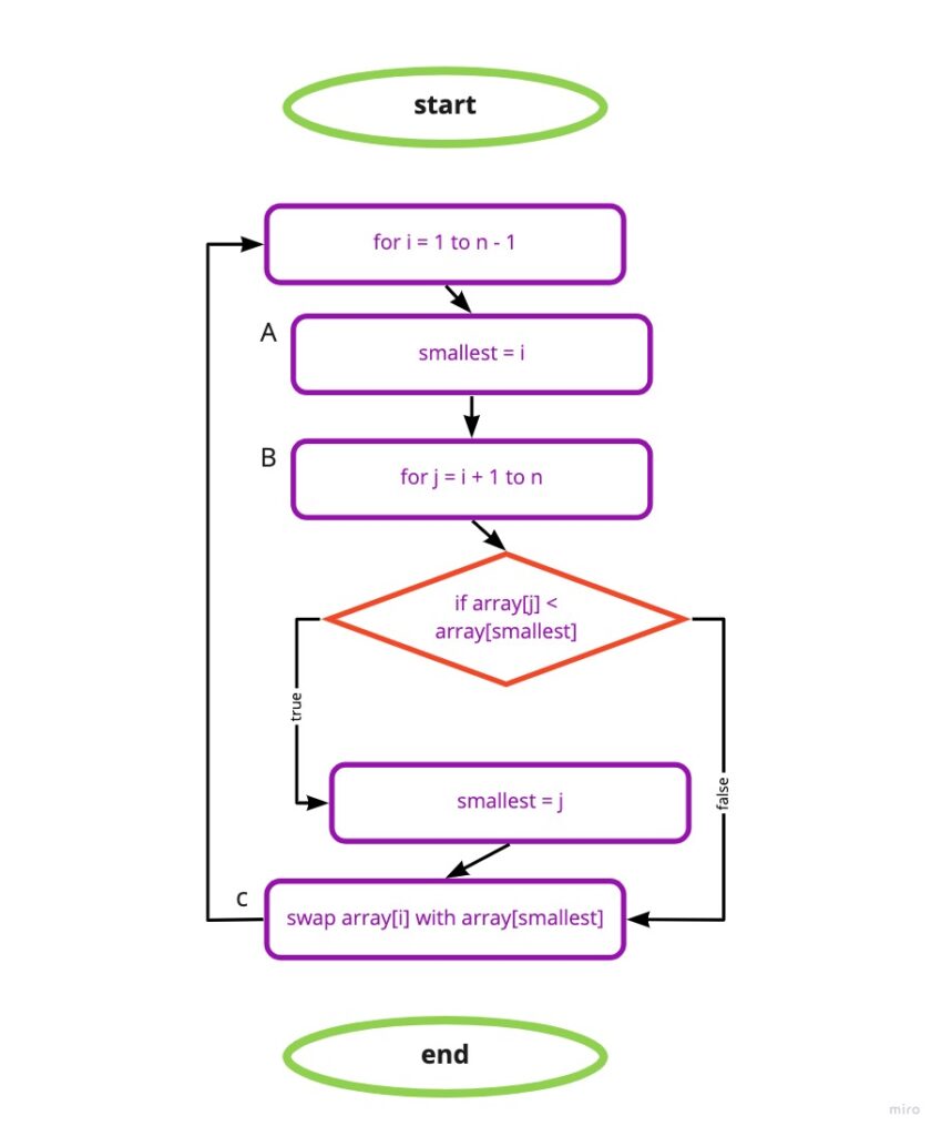
As we can see, the selectionSort procedure has a nested loop, with the loop of step 1B nested within the loop of step 1. The inner loop performs all of its iterations for every single iteration of the outer loop. The starting value of j in the inner loop depends on the current value of i in the outer loop. The algorithm ends up looking at ½(n2 – n) values where n is the number of elements in the array.
| Number of elements | Number of steps |
| 1 | 1 |
| 10 | 45 |
| 100 | 4950 |
| 1000 | 499500 |
| 10000 | 49995000 |
Exponential time
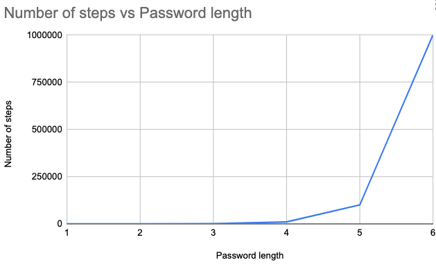
An algorithm’s run time is exponential if T(n) is bounded by O(2nk) for some constant k. When an algorithm grows in such superpolynomial time, its number of steps increases faster than a polynomial function of its input size.
For an example of an exponential time complexity algorithm, we could think of an algorithm that generates all possible numerical passwords given password length.
For a password length of 1, it will generate 10 passwords. If the length of the password is 2, we already have 100 possible passwords:
// passwords length = 2
[00, 01, ..., 99] // permutations = 100

// passwords length = 3
[000, 001, ... 999] // permutations = 1000
Let’s visit the growth of this function in a table:
| Password length | Permutations |
| 1 | 10 |
| 2 | 100 |
| 3 | 1000 |
| 4 | 10000 |
| 5 | 100000 |
Conclusion Polynomial vs. superpolynomial
The categories we’ve seen above are examples of runtime complexities for algorithms. The following graph (taken from the internet) compares them:
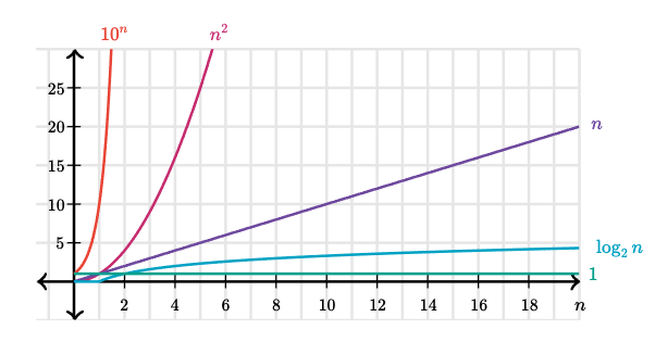
More running time categories can be broken into two classes: polynomial and superpolynomial.
- Polynomial time describes any run time that does not increase fater than nk, which includes constant time n0, logarithmic time log2 n, linear time n1, quadratic time n2, and other higher degree polynomials such as n3.
- Superpolynomial time describes any run time that does increase faster than nk, and includes exponential time 2n, factorial time n!, and anything else faster.
Big-O, Big-Theta, Big-Omega
These time categories can be asymptotically bound to the growth of a running time to within constant factors above and below. The below would mean the initiating variables, testing each element in the selection block, or returning a value. The above factors, the upper bound is the base iteration block of an algorithm, the steps that are directly bound to the input. As an input of an algorithm becomes very large, the lower bound of it becomes also important. Although, in this post, the running time categories of the algorithm used the Big-O notation – only the upper bound of an algorithm – here are short descriptions of Big-Theta and Big-Omega:
The metric that measures the growth of a running time to within constant factors above and below, is the big-Θ (Big-Theta) notation.
If we say that a running time is Θ(f(n)) in a particular situation, then it’s also O(f(n)). For example, we can say that because the worst-case running time of binary search is Θ(log2n), it’s also O(log2n)O.
The converse is not necessarily true: we can say that binary search always runs in O(log2n) time. But not that it always runs in Θ(log2n).
Another metric that measures only the lower bound of an algorithm, is the big-Ω (Big-Omega). If a running time is Ω(f(n)), then for large enough n, the running time is at least k⋅f(n) for some constant k.
We can also make correct, but imprecise statements using big-Ω notation. For example, if you have a million dollars in your pocket. You can truthfully say “I have an amount of money in my pocket, and it’s at least 10 dollars.” That is correct, but certainly not very precise. Similarly, we can correctly but imprecisely say that the worst-case running time of binary search is Ω(1) because we know that it takes at least constant time. But it doesn’t help much since in most cases it will take much more.